Differential expression analysis
Last updated on 2026-04-21 | Edit this page
Overview
Questions
- What transcriptomic changes do we observe in mouse models carrying AD-related mutations?
Objectives
- Read in a count matrix and metadata.
- Understand the data from AD mouse models
- Format the data for differential analysis
- Perform differential analysis using DESeq2.
- Pathway enrichment of differentially expressed genes
- Save data for next lessons
Differential Expression Analysis
WARNING
Warning: replacing previous import 'S4Arrays::makeNindexFromArrayViewport' by
'DelayedArray::makeNindexFromArrayViewport' when loading 'SummarizedExperiment'
Reading Gene Expression Count matrix from previous lesson
In this lesson, we will use the raw counts matrix and metadata downloaded in the previous lesson and will perform differential expression analysis.
R
counts <- read.delim("data/htseqcounts_5XFAD.txt",
                      check.names = FALSE)
Reading Sample Metadata from Previous Lesson
R
covars <- readRDS("data/covars_5XFAD.rds")
Let’s explore the data:
Let’s look at the top of the metadata.
R
head(covars)
OUTPUT
        individualID specimenID    sex         genotype timepoint
32043rh        32043    32043rh female    5XFAD_carrier     12 mo
32044rh        32044    32044rh   male 5XFAD_noncarrier     12 mo
32046rh        32046    32046rh   male 5XFAD_noncarrier     12 mo
32047rh        32047    32047rh   male 5XFAD_noncarrier     12 mo
32049rh        32049    32049rh female 5XFAD_noncarrier     12 mo
32057rh        32057    32057rh female 5XFAD_noncarrier     12 mo
identify distinct groups using sample metadata
R
distinct(covars, sex, genotype, timepoint)
OUTPUT
           sex         genotype timepoint
32043rh female    5XFAD_carrier     12 mo
32044rh   male 5XFAD_noncarrier     12 mo
32049rh female 5XFAD_noncarrier     12 mo
46105rh female 5XFAD_noncarrier      6 mo
46108rh   male 5XFAD_noncarrier      6 mo
46131rh female 5XFAD_noncarrier      4 mo
46877rh   male 5XFAD_noncarrier      4 mo
46887rh female    5XFAD_carrier      4 mo
32053rh   male    5XFAD_carrier     12 mo
46111rh female    5XFAD_carrier      6 mo
46865rh   male    5XFAD_carrier      6 mo
46866rh   male    5XFAD_carrier      4 mo
How many mice were used to produce this data?
R
covars %>%
  group_by(sex, genotype, timepoint) %>%
  dplyr::count()
OUTPUT
# A tibble: 12 × 4
# Groups:   sex, genotype, timepoint [12]
   sex    genotype         timepoint     n
   <chr>  <chr>            <chr>     <int>
 1 female 5XFAD_carrier    12 mo         6
 2 female 5XFAD_carrier    4 mo          6
 3 female 5XFAD_carrier    6 mo          6
 4 female 5XFAD_noncarrier 12 mo         6
 5 female 5XFAD_noncarrier 4 mo          6
 6 female 5XFAD_noncarrier 6 mo          6
 7 male   5XFAD_carrier    12 mo         6
 8 male   5XFAD_carrier    4 mo          6
 9 male   5XFAD_carrier    6 mo          6
10 male   5XFAD_noncarrier 12 mo         6
11 male   5XFAD_noncarrier 4 mo          6
12 male   5XFAD_noncarrier 6 mo          6
How many rows and columns are there in counts?
R
dim(counts)
OUTPUT
[1] 55489 73In the counts matrix, genes are in rows and samples are in columns. Let’s look at the first few rows.
R
head(counts, n=5)
OUTPUT
             gene_id 32043rh 32044rh 32046rh 32047rh 32048rh 32049rh 32050rh
1    ENSG00000080815   22554       0       0       0   16700       0       0
2    ENSG00000142192  344489       4       0       1  260935       6       8
3 ENSMUSG00000000001    5061    3483    3941    3088    2756    3067    2711
4 ENSMUSG00000000003       0       0       0       0       0       0       0
5 ENSMUSG00000000028     208     162     138     127      95     154     165
  32052rh 32053rh 32057rh 32059rh 32061rh 32062rh 32065rh 32067rh 32068rh
1   19748   14023       0   17062       0   15986      10       0   18584
2  337456  206851       1  264748       0  252248     172       4  300398
3    3334    3841    4068    3306    4076    3732    3940    4238    3257
4       0       0       0       0       0       0       0       0       0
5     124     103     164     116     108     134     204     239     148
  32070rh 32073rh 32074rh 32075rh 32078rh 32081rh 32088rh 32640rh 46105rh
1       1       0       0   22783   17029   16626   15573   12721       4
2       4       2       9  342655  280968  258597  243373  188818      19
3    3351    3449    4654    4844    3132    3334    3639    3355    4191
4       0       0       0       0       0       0       0       0       0
5     159     167     157     211     162     149     160     103     158
  46106rh 46107rh 46108rh 46109rh 46110rh 46111rh 46112rh 46113rh 46115rh
1       0       0       0       0       0   17931       0   19087       0
2       0       0       1       5       1  293409       8  273704       1
3    3058    4265    3248    3638    3747    3971    3192    3805    3753
4       0       0       0       0       0       0       0       0       0
5     167     199     113     168     175     203     158     108     110
  46121rh 46131rh 46132rh 46134rh 46138rh 46141rh 46142rh 46862rh 46863rh
1       0       0   12703   18833       0   18702   17666       0   14834
2       0       1  187975  285048       0  284499  250600       0  218494
3    4134    3059    3116    3853    3682    2844    3466    3442    3300
4       0       0       0       0       0       0       0       0       0
5     179     137     145     183     171     138      88     154     157
  46865rh 46866rh 46867rh 46868rh 46871rh 46872rh 46873rh 46874rh 46875rh
1   10546   10830   10316   10638   15248       0       0   11608   11561
2  169516  152769  151732  190150  229063       6       1  165941  171303
3    3242    3872    3656    3739    3473    3154    5510    3657    4121
4       0       0       0       0       0       0       0       0       0
5     131     152     152     155     140      80     240     148     112
  46876rh 46877rh 46878rh 46879rh 46881rh 46882rh 46883rh 46884rh 46885rh
1       0       0   12683   15613       0   14084   20753       0       0
2       0       2  183058  216122       0  199448  306081       0       5
3    3422    3829    3996    4324    2592    2606    4600    2913    3614
4       0       0       0       0       0       0       0       0       0
5     147     166     169     215     115     101     174     127     151
  46886rh 46887rh 46888rh 46889rh 46890rh 46891rh 46892rh 46893rh 46895rh
1   16639   16072       0   16680   13367       0   25119      92       0
2  242543  258061       0  235530  196721       0  371037    1116       0
3    3294    3719    3899    4173    4008    3037    5967    3459    4262
4       0       0       0       0       0       0       0       0       0
5     139     128     210     127     156     116     260     161     189
  46896rh 46897rh
1   15934       0
2  235343       6
3    3923    3486
4       0       0
5     179     117
As you can see, the gene ids are ENSEMBL IDs. There is some risk that these may not be unique. Let’s check whether any of the gene symbols are duplicated. We will sum the number of duplicated gene symbols.
R
sum(duplicated(rownames(counts)))
OUTPUT
[1] 0The sum equals zero, so there are no duplicated gene symbols, which is good. Similarly, samples should be unique. Once again, let’s verify this:
R
sum(duplicated(colnames(counts)))
OUTPUT
[1] 0Formatting the count matrix
Now, as we see that gene_id is in first column of count
matrix, but we will need only count data in matrix, so we will change
the gene_id column to rownames.
R
# Converting the `gene_id` as `rownames` of `counts` matrix
counts <- counts %>%
          column_to_rownames(., var = "gene_id") %>%
          as.data.frame()
Let’s confirm if change is done correctly.
R
head(counts, n=5)
OUTPUT
                   32043rh 32044rh 32046rh 32047rh 32048rh 32049rh 32050rh
ENSG00000080815      22554       0       0       0   16700       0       0
ENSG00000142192     344489       4       0       1  260935       6       8
ENSMUSG00000000001    5061    3483    3941    3088    2756    3067    2711
ENSMUSG00000000003       0       0       0       0       0       0       0
ENSMUSG00000000028     208     162     138     127      95     154     165
                   32052rh 32053rh 32057rh 32059rh 32061rh 32062rh 32065rh
ENSG00000080815      19748   14023       0   17062       0   15986      10
ENSG00000142192     337456  206851       1  264748       0  252248     172
ENSMUSG00000000001    3334    3841    4068    3306    4076    3732    3940
ENSMUSG00000000003       0       0       0       0       0       0       0
ENSMUSG00000000028     124     103     164     116     108     134     204
                   32067rh 32068rh 32070rh 32073rh 32074rh 32075rh 32078rh
ENSG00000080815          0   18584       1       0       0   22783   17029
ENSG00000142192          4  300398       4       2       9  342655  280968
ENSMUSG00000000001    4238    3257    3351    3449    4654    4844    3132
ENSMUSG00000000003       0       0       0       0       0       0       0
ENSMUSG00000000028     239     148     159     167     157     211     162
                   32081rh 32088rh 32640rh 46105rh 46106rh 46107rh 46108rh
ENSG00000080815      16626   15573   12721       4       0       0       0
ENSG00000142192     258597  243373  188818      19       0       0       1
ENSMUSG00000000001    3334    3639    3355    4191    3058    4265    3248
ENSMUSG00000000003       0       0       0       0       0       0       0
ENSMUSG00000000028     149     160     103     158     167     199     113
                   46109rh 46110rh 46111rh 46112rh 46113rh 46115rh 46121rh
ENSG00000080815          0       0   17931       0   19087       0       0
ENSG00000142192          5       1  293409       8  273704       1       0
ENSMUSG00000000001    3638    3747    3971    3192    3805    3753    4134
ENSMUSG00000000003       0       0       0       0       0       0       0
ENSMUSG00000000028     168     175     203     158     108     110     179
                   46131rh 46132rh 46134rh 46138rh 46141rh 46142rh 46862rh
ENSG00000080815          0   12703   18833       0   18702   17666       0
ENSG00000142192          1  187975  285048       0  284499  250600       0
ENSMUSG00000000001    3059    3116    3853    3682    2844    3466    3442
ENSMUSG00000000003       0       0       0       0       0       0       0
ENSMUSG00000000028     137     145     183     171     138      88     154
                   46863rh 46865rh 46866rh 46867rh 46868rh 46871rh 46872rh
ENSG00000080815      14834   10546   10830   10316   10638   15248       0
ENSG00000142192     218494  169516  152769  151732  190150  229063       6
ENSMUSG00000000001    3300    3242    3872    3656    3739    3473    3154
ENSMUSG00000000003       0       0       0       0       0       0       0
ENSMUSG00000000028     157     131     152     152     155     140      80
                   46873rh 46874rh 46875rh 46876rh 46877rh 46878rh 46879rh
ENSG00000080815          0   11608   11561       0       0   12683   15613
ENSG00000142192          1  165941  171303       0       2  183058  216122
ENSMUSG00000000001    5510    3657    4121    3422    3829    3996    4324
ENSMUSG00000000003       0       0       0       0       0       0       0
ENSMUSG00000000028     240     148     112     147     166     169     215
                   46881rh 46882rh 46883rh 46884rh 46885rh 46886rh 46887rh
ENSG00000080815          0   14084   20753       0       0   16639   16072
ENSG00000142192          0  199448  306081       0       5  242543  258061
ENSMUSG00000000001    2592    2606    4600    2913    3614    3294    3719
ENSMUSG00000000003       0       0       0       0       0       0       0
ENSMUSG00000000028     115     101     174     127     151     139     128
                   46888rh 46889rh 46890rh 46891rh 46892rh 46893rh 46895rh
ENSG00000080815          0   16680   13367       0   25119      92       0
ENSG00000142192          0  235530  196721       0  371037    1116       0
ENSMUSG00000000001    3899    4173    4008    3037    5967    3459    4262
ENSMUSG00000000003       0       0       0       0       0       0       0
ENSMUSG00000000028     210     127     156     116     260     161     189
                   46896rh 46897rh
ENSG00000080815      15934       0
ENSG00000142192     235343       6
ENSMUSG00000000001    3923    3486
ENSMUSG00000000003       0       0
ENSMUSG00000000028     179     117
As you can see from count table there are some genes that start with
ENSG and others start with ENSMUSG.
ENSG refers to human gene ENSEMBL id and
ENSMUSG refer to mouse ENSEMBL id. Let’s check how many
gene_ids are NOT from the mouse genome by searching for the
string “MUS” (as in Mus musculus) in the rownames
of the counts matrix.
R
counts[, 1:6] %>%
  filter(!str_detect(rownames(.), "MUS"))
OUTPUT
                32043rh 32044rh 32046rh 32047rh 32048rh 32049rh
ENSG00000080815   22554       0       0       0   16700       0
ENSG00000142192  344489       4       0       1  260935       6
Ok, so we see there are two human genes in out count matrix. Why? What genes are they?
Briefly, the 5xFAD mouse strain harbors two human transgenes APP
(ENSG00000142192) and PSEN1 (ENSG00000080815)
and inserted into exon 2 of the mouse Thy1 gene. To validate 5XFAD
strain and capture expression of human transgene APP and PS1, a custom
mouse genomic sequence was created and we quantified expression of human
as well as mouse App (ENSMUSG00000022892) and Psen1
(ENSMUSG00000019969) genes by our MODEL-AD RNA-Seq
pipeline.
Validation of 5xFAD mouse strain
First we convert the dataframe to longer format and join our
covariates by MouseID.
R
count_tpose <-  counts  %>%
                rownames_to_column(., var = "gene_id") %>%
                filter(gene_id %in%
                      c("ENSG00000080815",
                        "ENSMUSG00000019969",
                        "ENSG00000142192",
                        "ENSMUSG00000022892")) %>%
                pivot_longer(., cols    = -"gene_id",
                              names_to  = "specimenID",
                              values_to = "counts") %>%
                as.data.frame() %>%
                left_join(covars, by="specimenID") %>%
                as.data.frame()

head(count_tpose)
OUTPUT
          gene_id specimenID counts individualID    sex         genotype
1 ENSG00000080815    32043rh  22554        32043 female    5XFAD_carrier
2 ENSG00000080815    32044rh      0        32044   male 5XFAD_noncarrier
3 ENSG00000080815    32046rh      0        32046   male 5XFAD_noncarrier
4 ENSG00000080815    32047rh      0        32047   male 5XFAD_noncarrier
5 ENSG00000080815    32048rh  16700        32048 female    5XFAD_carrier
6 ENSG00000080815    32049rh      0        32049 female 5XFAD_noncarrier
  timepoint
1     12 mo
2     12 mo
3     12 mo
4     12 mo
5     12 mo
6     12 mo
Rename the APP and PSEN1 genes to specify whether mouse or human.
R
# make the age column a factor and re-order the levels
count_tpose$timepoint <- factor(count_tpose$timepoint,
                                levels = c("4 mo", "6 mo", "12 mo"))

# rename the gene id to gene symbol
count_tpose$gene_id[count_tpose$gene_id %in% "ENSG00000142192"] <-
  "Human APP"
count_tpose$gene_id[count_tpose$gene_id %in% "ENSG00000080815"] <-
  "Human PSEN1"
count_tpose$gene_id[count_tpose$gene_id %in% "ENSMUSG00000022892"] <-
  "Mouse App"
count_tpose$gene_id[count_tpose$gene_id %in% "ENSMUSG00000019969"] <-
  "Mouse Psen1"
Visualize orthologous genes.
R
# Create simple box plots showing normalized counts
# by genotype and time point faceted by sex.
count_tpose %>%
  ggplot(aes(x = timepoint, y = counts, color = genotype)) +
        geom_boxplot() +
        geom_point(position = position_jitterdodge()) +
        facet_wrap(~ sex + gene_id) +
        theme_bw()
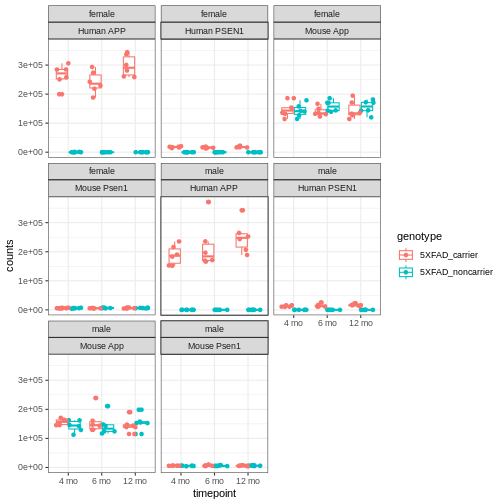
You will notice expression of Human APP is higher in 5XFAD carriers but lower in non-carriers. However mouse App expressed in both 5XFAD carrier and non-carrier.
We are going to sum the counts from both orthologous genes (human APP and mouse App; human PSEN1 and mouse Psen1) and save the summed expression as expression of mouse genes, respectively to match with gene names in control mice.
R
# merge mouse and human APP gene raw count
counts[rownames(counts)   %in% "ENSMUSG00000022892", ] <-
  counts[rownames(counts) %in% "ENSMUSG00000022892", ] +
  counts[rownames(counts) %in% "ENSG00000142192", ]

counts <- counts[!rownames(counts) %in% c("ENSG00000142192"), ]

# merge mouse and human PS1 gene raw count
counts[rownames(counts)   %in% "ENSMUSG00000019969", ] <-
  counts[rownames(counts) %in% "ENSMUSG00000019969", ] +
  counts[rownames(counts) %in% "ENSG00000080815", ]

counts <- counts[!rownames(counts) %in% c("ENSG00000080815"), ]
Let’s verify if expression of both human genes have been merged or not:
R
counts[, 1:6] %>%
  filter(!str_detect(rownames(.), "MUS"))
OUTPUT
[1] 32043rh 32044rh 32046rh 32047rh 32048rh 32049rh
<0 rows> (or 0-length row.names)
What proportion of genes have zero counts in all samples?
R
gene_sums <- data.frame(gene_id = rownames(counts),
                        sums    = Matrix::rowSums(counts))
sum(gene_sums$sums == 0)
OUTPUT
[1] 9691We can see that 9,691 (17%) genes have no reads at all associated with them. In the next lesson, we will remove genes that have no counts in any samples.
Differential Analysis using DESeq2
Now, after exploring and formatting the data, We will look for differential expression between the control and 5xFAD mice at different ages for both sexes. The differentially expressed genes (DEGs) can inform our understanding of how the 5XFAD mutation affects biological processes.
DESeq2 analysis consist of multiple steps. We are going to briefly understand some of the important steps using a subset of data and then we will perform differential analysis on the whole dataset.
First, order the data (so counts and metadata specimenID
orders match) and save as another variable name.
R
rawdata  <- counts[, sort(colnames(counts))]
metadata <- covars[sort(rownames(covars)), ]
Subset the counts matrix and sample metadata to include only 12-month old male mice. You can amend the code to compare wild type and 5XFAD mice from either sex, at any time point.
R
meta.12M.Male <- metadata[(metadata$sex           == "male" &
                           metadata$timepoint     == "12 mo"), ]

meta.12M.Male
OUTPUT
        individualID specimenID  sex         genotype timepoint
32044rh        32044    32044rh male 5XFAD_noncarrier     12 mo
32046rh        32046    32046rh male 5XFAD_noncarrier     12 mo
32047rh        32047    32047rh male 5XFAD_noncarrier     12 mo
32053rh        32053    32053rh male    5XFAD_carrier     12 mo
32059rh        32059    32059rh male    5XFAD_carrier     12 mo
32061rh        32061    32061rh male 5XFAD_noncarrier     12 mo
32062rh        32062    32062rh male    5XFAD_carrier     12 mo
32073rh        32073    32073rh male 5XFAD_noncarrier     12 mo
32074rh        32074    32074rh male 5XFAD_noncarrier     12 mo
32075rh        32075    32075rh male    5XFAD_carrier     12 mo
32088rh        32088    32088rh male    5XFAD_carrier     12 mo
32640rh        32640    32640rh male    5XFAD_carrier     12 mo
R
dat <- as.matrix(rawdata[ , colnames(rawdata) %in%
                            rownames(meta.12M.Male)])
colnames(dat)
OUTPUT
 [1] "32044rh" "32046rh" "32047rh" "32053rh" "32059rh" "32061rh" "32062rh"
 [8] "32073rh" "32074rh" "32075rh" "32088rh" "32640rh"
R
rownames(meta.12M.Male)
OUTPUT
 [1] "32044rh" "32046rh" "32047rh" "32053rh" "32059rh" "32061rh" "32062rh"
 [8] "32073rh" "32074rh" "32075rh" "32088rh" "32640rh"
R
match(colnames(dat), rownames(meta.12M.Male))
OUTPUT
[1] 1 2 3 4 5 6 7 8 9 10 11 12Next, we build the DESeqDataSet using the following
function:
R
ddsHTSeq <- DESeqDataSetFromMatrix(countData = dat,
                                   colData   = meta.12M.Male,
                                   design    = ~ genotype)
WARNING
Warning in DESeqDataSet(se, design = design, ignoreRank): some variables in
design formula are characters, converting to factors
R
ddsHTSeq
OUTPUT
class: DESeqDataSet
dim: 55487 12
metadata(1): version
assays(1): counts
rownames(55487): ENSMUSG00000000001 ENSMUSG00000000003 ...
  ENSMUSG00000118487 ENSMUSG00000118488
rowData names(0):
colnames(12): 32044rh 32046rh ... 32088rh 32640rh
colData names(5): individualID specimenID sex genotype timepoint
Pre-filtering
While it is not necessary to pre-filter low count genes before running the DESeq2 functions, there are two reasons which make pre-filtering useful: by removing rows in which there are very few reads, we reduce the memory size of the dds data object, and we increase the speed of the transformation and testing functions within DESeq2. It can also improve visualizations, as features with no information for differential expression are not plotted.
Here we perform a minimal pre-filtering to keep only rows that have at least 10 reads total.
R
ddsHTSeq <- ddsHTSeq[rowSums(counts(ddsHTSeq)) >= 10, ]

ddsHTSeq
OUTPUT
class: DESeqDataSet
dim: 33059 12
metadata(1): version
assays(1): counts
rownames(33059): ENSMUSG00000000001 ENSMUSG00000000028 ...
  ENSMUSG00000118486 ENSMUSG00000118487
rowData names(0):
colnames(12): 32044rh 32046rh ... 32088rh 32640rh
colData names(5): individualID specimenID sex genotype timepoint
Reference level
By default, R will choose a reference level for factors based on
alphabetical order. Then, if you never tell the DESeq2
functions which level you want to compare against (e.g. which
level represents the control group), the comparisons will be based on
the alphabetical order of the levels.
R
# specifying the reference-level to `5XFAD_noncarrier`
ddsHTSeq$genotype <- relevel(ddsHTSeq$genotype, ref = "5XFAD_noncarrier")
Run the standard differential expression analysis steps that is
wrapped into a single function, DESeq.
R
dds <- DESeq(ddsHTSeq, parallel = TRUE)
OUTPUT
estimating size factorsOUTPUT
estimating dispersionsOUTPUT
gene-wise dispersion estimates: 2 workersOUTPUT
mean-dispersion relationshipOUTPUT
final dispersion estimates, fitting model and testing: 2 workersResults tables are generated using the function results, which
extracts a results table with log2 fold changes, p-values and adjusted
p-values. By default the argument alpha is set to 0.1. If
the adjusted p-value cutoff will be a value other than 0.1, alpha should
be set to that value:
R
res <- results(dds, alpha=0.05)  # setting 0.05 as significant threshold
res
OUTPUT
log2 fold change (MLE): genotype 5XFAD carrier vs 5XFAD noncarrier
Wald test p-value: genotype 5XFAD carrier vs 5XFAD noncarrier
DataFrame with 33059 rows and 6 columns
                    baseMean log2FoldChange     lfcSE      stat    pvalue
                   <numeric>      <numeric> <numeric> <numeric> <numeric>
ENSMUSG00000000001 3737.9009      0.0148125 0.0466948  0.317219 0.7510777
ENSMUSG00000000028  138.5635     -0.0712500 0.1550131 -0.459639 0.6457754
ENSMUSG00000000031   29.2983      0.6705922 0.3563442  1.881866 0.0598541
ENSMUSG00000000037  123.6482     -0.2184054 0.1554362 -1.405113 0.1599876
ENSMUSG00000000049   15.1733      0.3657555 0.3924376  0.932010 0.3513316
...                      ...            ...       ...       ...       ...
ENSMUSG00000118473   1.18647      -0.377971  1.531586 -0.246784  0.805075
ENSMUSG00000118477  59.10359      -0.144081  0.226690 -0.635586  0.525046
ENSMUSG00000118479  24.64566      -0.181992  0.341445 -0.533006  0.594029
ENSMUSG00000118486   1.92048       0.199838  1.253875  0.159376  0.873372
ENSMUSG00000118487  65.78311      -0.191362  0.218593 -0.875427  0.381342
                        padj
                   <numeric>
ENSMUSG00000000001  0.943421
ENSMUSG00000000028  0.913991
ENSMUSG00000000031  0.352346
ENSMUSG00000000037  0.566360
ENSMUSG00000000049  0.765640
...                      ...
ENSMUSG00000118473        NA
ENSMUSG00000118477  0.863565
ENSMUSG00000118479  0.893356
ENSMUSG00000118486        NA
ENSMUSG00000118487  0.785846
We can order our results table by the smallest p-value:
R
resOrdered <- res[order(res$pvalue), ]

head(resOrdered, n=10)
OUTPUT
log2 fold change (MLE): genotype 5XFAD carrier vs 5XFAD noncarrier
Wald test p-value: genotype 5XFAD carrier vs 5XFAD noncarrier
DataFrame with 10 rows and 6 columns
                     baseMean log2FoldChange     lfcSE      stat       pvalue
                    <numeric>      <numeric> <numeric> <numeric>    <numeric>
ENSMUSG00000019969  13860.942        1.90740 0.0432685   44.0828  0.00000e+00
ENSMUSG00000030579   2367.096        2.61215 0.0749326   34.8600 2.99982e-266
ENSMUSG00000046805   7073.296        2.12247 0.0635035   33.4229 6.38461e-245
ENSMUSG00000032011  80423.476        1.36195 0.0424007   32.1210 2.24203e-226
ENSMUSG00000022892 271265.838        1.36140 0.0434167   31.3567 7.88742e-216
ENSMUSG00000038642  10323.969        1.69717 0.0549488   30.8864 1.81875e-209
ENSMUSG00000023992   2333.227        2.62290 0.0882819   29.7105 5.61838e-194
ENSMUSG00000079293    761.313        5.12514 0.1738382   29.4822 4.86644e-191
ENSMUSG00000040552    617.149        2.22726 0.0781799   28.4889 1.60609e-178
ENSMUSG00000069516   2604.926        2.34471 0.0847390   27.6697 1.61630e-168
                           padj
                      <numeric>
ENSMUSG00000019969  0.00000e+00
ENSMUSG00000030579 3.60954e-262
ENSMUSG00000046805 5.12152e-241
ENSMUSG00000032011 1.34886e-222
ENSMUSG00000022892 3.79622e-212
ENSMUSG00000038642 7.29469e-206
ENSMUSG00000023992 1.93152e-190
ENSMUSG00000079293 1.46389e-187
ENSMUSG00000040552 4.29450e-175
ENSMUSG00000069516 3.88961e-165
We can summarize some basic tallies using the summary function.
R
summary(res)
OUTPUT
out of 33059 with nonzero total read count
adjusted p-value < 0.05
LFC > 0 (up)       : 1098, 3.3%
LFC < 0 (down)     : 505, 1.5%
outliers [1]       : 33, 0.1%
low counts [2]     : 8961, 27%
(mean count < 8)
[1] see 'cooksCutoff' argument of ?results
[2] see 'independentFiltering' argument of ?results
How many adjusted p-values were less than 0.05?
R
sum(res$padj < 0.05, na.rm=TRUE)
OUTPUT
[1] 1603How many adjusted p-values were less than 0.1?
R
sum(res$padj < 0.1, na.rm=TRUE)
OUTPUT
[1] 2001Function to convert ensembleIDs to common gene names
We’ll use a package to translate mouse ENSEMBL IDS to gene names. Run this function and they will be called up when assembling results from the differential expression analysis.
R
map_function.df <- function(x, inputtype, outputtype) {
                            mapIds( org.Mm.eg.db,
                                    keys      = row.names(x),
                                    column    = outputtype,
                                    keytype   = inputtype,
                                    multiVals = "first")
                            }
Generating Results table
Here we will call the function to get the symbol names
of the genes incorporated into the results table, along with the columns
we are most interested in.
R
All_res <- as.data.frame(res) %>%

           # run map_function to add symbol of gene corresponding to ENSEMBL ID
           mutate(symbol = map_function.df(res, "ENSEMBL", "SYMBOL")) %>%

           # run map_function to add Entrez ID of gene corresponding to ENSEMBL ID
           mutate(EntrezGene = map_function.df(res, "ENSEMBL", "ENTREZID")) %>%
           dplyr::select("symbol",
                         "EntrezGene",
                         "baseMean",
                         "log2FoldChange",
                         "lfcSE",
                         "stat",
                         "pvalue",
                         "padj")
OUTPUT
'select()' returned 1:many mapping between keys and columns
'select()' returned 1:many mapping between keys and columns
R
head(All_res)
OUTPUT
                   symbol EntrezGene   baseMean log2FoldChange      lfcSE
ENSMUSG00000000001  Gnai3      14679 3737.90089     0.01481247 0.04669481
ENSMUSG00000000028  Cdc45      12544  138.56354    -0.07125004 0.15501305
ENSMUSG00000000031    H19      14955   29.29832     0.67059217 0.35634418
ENSMUSG00000000037  Scml2     107815  123.64823    -0.21840544 0.15543617
ENSMUSG00000000049   Apoh      11818   15.17325     0.36575555 0.39243756
ENSMUSG00000000056   Narf      67608 5017.30216    -0.06713961 0.04466809
                         stat     pvalue      padj
ENSMUSG00000000001  0.3172187 0.75107766 0.9434210
ENSMUSG00000000028 -0.4596390 0.64577537 0.9139907
ENSMUSG00000000031  1.8818665 0.05985415 0.3523459
ENSMUSG00000000037 -1.4051134 0.15998756 0.5663602
ENSMUSG00000000049  0.9320095 0.35133160 0.7656400
ENSMUSG00000000056 -1.5030778 0.13281898 0.5203335
Extracting genes that are significantly expressed
Let’s subset all the genes with a p-value < 0.05.
R
dseq_res <- subset(All_res[order(All_res$padj), ], padj < 0.05)
Wow! We have a lot of genes with apparently very strong statistically significant differences between the control and 5xFAD carrier.
R
dim(dseq_res)
OUTPUT
[1] 1603 8R
head(dseq_res)
OUTPUT
                   symbol EntrezGene   baseMean log2FoldChange      lfcSE
ENSMUSG00000019969  Psen1      19164  13860.942       1.907397 0.04326854
ENSMUSG00000030579 Tyrobp      22177   2367.096       2.612152 0.07493257
ENSMUSG00000046805  Mpeg1      17476   7073.296       2.122467 0.06350348
ENSMUSG00000032011   Thy1      21838  80423.476       1.361953 0.04240065
ENSMUSG00000022892    App      11820 271265.838       1.361405 0.04341673
ENSMUSG00000038642   Ctss      13040  10323.969       1.697172 0.05494883
                       stat        pvalue          padj
ENSMUSG00000019969 44.08277  0.000000e+00  0.000000e+00
ENSMUSG00000030579 34.86004 2.999825e-266 3.609539e-262
ENSMUSG00000046805 33.42285 6.384608e-245 5.121519e-241
ENSMUSG00000032011 32.12104 2.242032e-226 1.348863e-222
ENSMUSG00000022892 31.35669 7.887422e-216 3.796216e-212
ENSMUSG00000038642 30.88640 1.818747e-209 7.294691e-206
Exploring and exporting results
Exporting results to CSV files
We can save results file into a csv file like this:
R
write.csv(All_res, file="results/All_5xFAD_12months_male.csv")
write.csv(dseq_res, file="results/DEG_5xFAD_12months_male.csv")
Volcano plot
We can visualize the differential expression results using the
volcano plot function from EnhancedVolcano package. For the
most basic volcano plot, only a single data frame, data matrix, or
tibble of test results is required, containing point labels, log2FC, and
adjusted or unadjusted p-values. The default cut-off for log2FC is
>|2|; the default cut-off for p-value is 10e-6.
R
EnhancedVolcano(All_res,
                lab            = (All_res$symbol),
                x              = 'log2FoldChange',
                y              = 'padj',
                legendPosition = 'none',
                title          = 'Volcano plot:Differential Expression Results',
                subtitle       = '',
                FCcutoff       = 0.1,
                pCutoff        = 0.05,
                xlim           = c(-3, 6))
WARNING
Warning: One or more p-values is 0. Converting to 10^-1 * current lowest
non-zero p-value...
WARNING
Warning: Using `size` aesthetic for lines was deprecated in ggplot2 3.4.0.
ℹ Please use `linewidth` instead.
ℹ The deprecated feature was likely used in the EnhancedVolcano package.
  Please report the issue to the authors.
This warning is displayed once per session.
Call `lifecycle::last_lifecycle_warnings()` to see where this warning was
generated.
WARNING
Warning: The `size` argument of `element_line()` is deprecated as of ggplot2 3.4.0.
ℹ Please use the `linewidth` argument instead.
ℹ The deprecated feature was likely used in the EnhancedVolcano package.
  Please report the issue to the authors.
This warning is displayed once per session.
Call `lifecycle::last_lifecycle_warnings()` to see where this warning was
generated.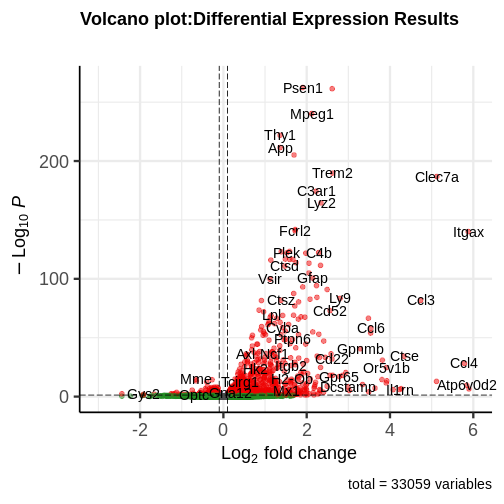
You can see that some top significantly expressed are immune/inflammation-related genes such as Ctsd, C4b, Csf1 etc. These genes are upregulated in the 5XFAD strain.
Principal component plot of the samples
Principal component analysis is a dimension reduction technique that reduces the dimensionality of these large matrixes into a linear coordinate system, so that we can more easily visualize what factors are contributing the most to variation in the dataset by graphing the principal components.
R
ddsHTSeq <- DESeqDataSetFromMatrix(countData = as.matrix(rawdata),
                                   colData   = metadata,
                                   design    = ~ genotype)
WARNING
Warning in DESeqDataSet(se, design = design, ignoreRank): some variables in
design formula are characters, converting to factors
R
ddsHTSeq <- ddsHTSeq[rowSums(counts(ddsHTSeq) > 1) >= 10, ]
dds <- DESeq(ddsHTSeq, parallel = TRUE)
OUTPUT
estimating size factorsOUTPUT
estimating dispersionsOUTPUT
gene-wise dispersion estimates: 2 workersOUTPUT
mean-dispersion relationshipOUTPUT
final dispersion estimates, fitting model and testing: 2 workersOUTPUT
-- replacing outliers and refitting for 42 genes
-- DESeq argument 'minReplicatesForReplace' = 7
-- original counts are preserved in counts(dds)
OUTPUT
estimating dispersionsOUTPUT
fitting model and testingR
vsd <- varianceStabilizingTransformation(dds, blind = FALSE)
plotPCA(vsd, intgroup = c("genotype", "sex", "timepoint"))
OUTPUT
using ntop=500 top features by variance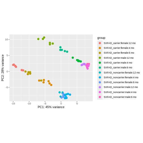
We can see that clustering is occurring, though it’s kind of hard to see exactly how they are clustering in this visualization.
It is also possible to customize the PCA plot using the
ggplot function.
R
pcaData <- plotPCA(vsd,
                   intgroup   = c("genotype", "sex","timepoint"),
                   returnData = TRUE)
OUTPUT
using ntop=500 top features by varianceR
percentVar <- round(100 * attr(pcaData, "percentVar"))

ggplot(pcaData, aes(PC1, PC2,color = genotype, shape = sex)) +
       geom_point(size=3) +
       geom_text(aes(label = timepoint), hjust=0.5, vjust=2, size =3.5) +
       labs(x = paste0("PC1: ", percentVar[1], "% variance"),
            y = paste0("PC2: ", percentVar[2], "% variance"))
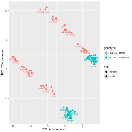
PCA identified genotype and sex being a major source of variation in between 5XFAD and WT mice. Female and male samples from the 5XFAD carriers clustered distinctly at all ages, suggesting the presence of sex-biased molecular changes in animals.
Function for Differential analysis using DESeq2
Finally, we can build a function for differential analysis that consists of all above discussed steps. It will require to input sorted raw count matrix, sample metadata and define the reference group.
R
DEG <- function(rawdata, meta, include.batch = FALSE, ref = ref) {
                dseq_res <- data.frame()
                All_res  <- data.frame()

                if (include.batch) {
                    cat("Including batch as covariate\n")
                    design_formula <- ~ Batch + genotype
                    }
                else {
                    design_formula <- ~ genotype
                    }

                dat2 <- as.matrix(rawdata[, colnames(rawdata) %in%
                                            rownames(meta)])

                ddsHTSeq <- DESeqDataSetFromMatrix(countData = dat2,
                            colData = meta,
                            design = design_formula)

                ddsHTSeq <- ddsHTSeq[rowSums(counts(ddsHTSeq)) >= 10, ]

                ddsHTSeq$genotype <- relevel(ddsHTSeq$genotype, ref = ref)

                dds <- DESeq(ddsHTSeq, parallel = TRUE)

                res <- results(dds, alpha = 0.05)
                #summary(res)

                res$symbol <- map_function.df(res,"ENSEMBL","SYMBOL")

                res$EntrezGene <- map_function.df(res,"ENSEMBL","ENTREZID")

                All_res <<- as.data.frame(res[, c("symbol",
                                                  "EntrezGene",
                                                  "baseMean",
                                                  "log2FoldChange",
                                                  "lfcSE",
                                                  "stat",
                                                  "pvalue",
                                                  "padj")])
              }
Let’s use this function to analyze all groups present in our data.
Differential Analysis of all groups
First, we add a Group column to our metadata table that
will combine all variables of interest (genotype,
sex, and timepoint) for each sample.
R
metadata$Group <- paste0(metadata$genotype,
                         "-",
                         metadata$sex,
                         "-",
                         metadata$timepoint)
unique(metadata$Group)
OUTPUT
 [1] "5XFAD_carrier-female-12 mo"    "5XFAD_noncarrier-male-12 mo"
 [3] "5XFAD_noncarrier-female-12 mo" "5XFAD_carrier-male-12 mo"
 [5] "5XFAD_noncarrier-female-6 mo"  "5XFAD_noncarrier-male-6 mo"
 [7] "5XFAD_carrier-female-6 mo"     "5XFAD_noncarrier-female-4 mo"
 [9] "5XFAD_carrier-female-4 mo"     "5XFAD_carrier-male-6 mo"
[11] "5XFAD_carrier-male-4 mo"       "5XFAD_noncarrier-male-4 mo"
Next, we create a comparison table that has all cases and controls that we would like to compare with each other. Here I have made comparison groups for age and sex-matched 5xFAD carriers vs 5xFAD_noncarriers, with carriers as the cases and noncarriers as the controls:
R
comparisons <-  data.frame(control = c("5XFAD_noncarrier-male-4 mo",
                                       "5XFAD_noncarrier-female-4 mo",
                                       "5XFAD_noncarrier-male-6 mo",
                                       "5XFAD_noncarrier-female-6 mo",
                                       "5XFAD_noncarrier-male-12 mo",
                                       "5XFAD_noncarrier-female-12 mo"),
                           case    = c("5XFAD_carrier-male-4 mo",
                                       "5XFAD_carrier-female-4 mo",
                                       "5XFAD_carrier-male-6 mo",
                                       "5XFAD_carrier-female-6 mo",
                                       "5XFAD_carrier-male-12 mo",
                                       "5XFAD_carrier-female-12 mo"))
R
comparisons
OUTPUT
                        control                       case
1    5XFAD_noncarrier-male-4 mo    5XFAD_carrier-male-4 mo
2  5XFAD_noncarrier-female-4 mo  5XFAD_carrier-female-4 mo
3    5XFAD_noncarrier-male-6 mo    5XFAD_carrier-male-6 mo
4  5XFAD_noncarrier-female-6 mo  5XFAD_carrier-female-6 mo
5   5XFAD_noncarrier-male-12 mo   5XFAD_carrier-male-12 mo
6 5XFAD_noncarrier-female-12 mo 5XFAD_carrier-female-12 mo
Finally, we implement our DEG function on each
case/control comparison of interest and store the result table in a list
and data frame:
R
# initiate an empty list and data frame to save results
DE_5xFAD.list <- list()
DE_5xFAD.df   <- data.frame()

for (i in 1:nrow(comparisons))
  {
    meta <- metadata[metadata$Group %in% comparisons[i,],]
    DEG(rawdata, meta, ref = "5XFAD_noncarrier")

    # append results in data frame
    DE_5xFAD.df <- rbind(DE_5xFAD.df,
                         All_res %>%
                         mutate(model = "5xFAD",
                                sex   = unique(meta$sex),
                                age   = unique(meta$timepoint)))

    # append results in list
    DE_5xFAD.list[[i]] <- All_res
    names(DE_5xFAD.list)[i] <- paste0(comparisons[i,2])
}
WARNING
Warning in DESeqDataSet(se, design = design, ignoreRank): some variables in
design formula are characters, converting to factors
OUTPUT
estimating size factorsOUTPUT
estimating dispersionsOUTPUT
gene-wise dispersion estimates: 2 workersOUTPUT
mean-dispersion relationshipOUTPUT
final dispersion estimates, fitting model and testing: 2 workersOUTPUT
'select()' returned 1:many mapping between keys and columns
'select()' returned 1:many mapping between keys and columns
Let’s explore the result stored in our list:
R
names(DE_5xFAD.list)
OUTPUT
[1] "5XFAD_carrier-male-4 mo"    "5XFAD_carrier-female-4 mo"
[3] "5XFAD_carrier-male-6 mo"    "5XFAD_carrier-female-6 mo"
[5] "5XFAD_carrier-male-12 mo"   "5XFAD_carrier-female-12 mo"
We can easily extract the result table for any group of interest by
using $ and name of group. Let’s check top few rows from
5XFAD_carrier-male-4 mo group:
R
head(DE_5xFAD.list$`5XFAD_carrier-male-4 mo`)
OUTPUT
                   symbol EntrezGene   baseMean log2FoldChange      lfcSE
ENSMUSG00000000001  Gnai3      14679 3707.53159   -0.023085867 0.03816431
ENSMUSG00000000028  Cdc45      12544  159.76225   -0.009444942 0.13226126
ENSMUSG00000000031    H19      14955   35.96987    0.453401511 0.27852555
ENSMUSG00000000037  Scml2     107815  126.82414    0.089394568 0.13774048
ENSMUSG00000000049   Apoh      11818   19.99721    0.115325773 0.31548606
ENSMUSG00000000056   Narf      67608 5344.21741   -0.100413295 0.03811800
                          stat      pvalue      padj
ENSMUSG00000000001 -0.60490724 0.545240632 0.9999514
ENSMUSG00000000028 -0.07141125 0.943070457 0.9999514
ENSMUSG00000000031  1.62786329 0.103553876 0.9999514
ENSMUSG00000000037  0.64900725 0.516333691 0.9999514
ENSMUSG00000000049  0.36554951 0.714701258 0.9999514
ENSMUSG00000000056 -2.63427474 0.008431723 0.5696567
Let’s check the result stored as dataframe:
R
head(DE_5xFAD.df)
OUTPUT
                   symbol EntrezGene   baseMean log2FoldChange      lfcSE
ENSMUSG00000000001  Gnai3      14679 3707.53159   -0.023085867 0.03816431
ENSMUSG00000000028  Cdc45      12544  159.76225   -0.009444942 0.13226126
ENSMUSG00000000031    H19      14955   35.96987    0.453401511 0.27852555
ENSMUSG00000000037  Scml2     107815  126.82414    0.089394568 0.13774048
ENSMUSG00000000049   Apoh      11818   19.99721    0.115325773 0.31548606
ENSMUSG00000000056   Narf      67608 5344.21741   -0.100413295 0.03811800
                          stat      pvalue      padj model  sex  age
ENSMUSG00000000001 -0.60490724 0.545240632 0.9999514 5xFAD male 4 mo
ENSMUSG00000000028 -0.07141125 0.943070457 0.9999514 5xFAD male 4 mo
ENSMUSG00000000031  1.62786329 0.103553876 0.9999514 5xFAD male 4 mo
ENSMUSG00000000037  0.64900725 0.516333691 0.9999514 5xFAD male 4 mo
ENSMUSG00000000049  0.36554951 0.714701258 0.9999514 5xFAD male 4 mo
ENSMUSG00000000056 -2.63427474 0.008431723 0.5696567 5xFAD male 4 mo
Check if result is present for all ages:
R
unique((DE_5xFAD.df$age))
OUTPUT
[1] "4 mo" "6 mo" "12 mo"Check if result is present for both sexes:
R
unique((DE_5xFAD.df$sex))
OUTPUT
[1] "male" "female"Check number of genes in each group:
R
dplyr::count(DE_5xFAD.df, model, sex, age)
OUTPUT
  model    sex   age     n
1 5xFAD female 12 mo 33120
2 5xFAD female  4 mo 32930
3 5xFAD female  6 mo 33249
4 5xFAD   male 12 mo 33059
5 5xFAD   male  4 mo 33119
6 5xFAD   male  6 mo 33375
Check number of genes significantly differentially expressed in all cases compared to age and sex-matched controls:
R
degs.up <- map(DE_5xFAD.list,
               ~ length(which(.x$padj          < 0.05 &
                             .x$log2FoldChange > 0)))

degs.down <- map(DE_5xFAD.list,
                 ~ length(which(.x$padj           < 0.05 &
                                .x$log2FoldChange < 0)))

deg <- data.frame(Case              = names(degs.up),
                  Up_DEGs.pval.05   = as.vector(unlist(degs.up)),
                  Down_DEGs.pval.05 = as.vector(unlist(degs.down)))

knitr::kable(deg)
| Case | Up_DEGs.pval.05 | Down_DEGs.pval.05 |
|---|---|---|
| 5XFAD_carrier-male-4 mo | 86 | 11 |
| 5XFAD_carrier-female-4 mo | 522 | 90 |
| 5XFAD_carrier-male-6 mo | 714 | 488 |
| 5XFAD_carrier-female-6 mo | 1081 | 409 |
| 5XFAD_carrier-male-12 mo | 1098 | 505 |
| 5XFAD_carrier-female-12 mo | 1494 | 1023 |
Interestingly, in females more genes are differentially expressed at all age groups, and more genes are differentially expressed the older the mice get in both sexes.
Pathway Enrichment
We may wish to look for enrichment of biological pathways in a list
of differentially expressed genes. Here we will test for enrichment of
KEGG pathways using using the enrichKEGG function in the
clusterProfiler package.
R
dat <- list(FAD_M_4 = subset(DE_5xFAD.list$`5XFAD_carrier-male-4 mo`[order(DE_5xFAD.list$`5XFAD_carrier-male-4 mo`$padj), ],
                             padj < 0.05) %>%
            pull(EntrezGene),
                 FAD_F_4 = subset(DE_5xFAD.list$`5XFAD_carrier-female-4 mo`[order(DE_5xFAD.list$`5XFAD_carrier-female-4 mo`$padj), ],
                                  padj < 0.05) %>%
            pull(EntrezGene))

# perform enrichment analysis
enrich_pathway <- compareCluster(dat,
                                 fun          = "enrichKEGG",
                                 pvalueCutoff = 0.05,
                                 organism     = "mmu"
                                 )

enrich_pathway@compareClusterResult$Description <-
                          gsub(" - Mus musculus \\(house mouse)",
                               "",
                               enrich_pathway@compareClusterResult$Description)
Let’s plot top enriched functions using the dotplot
function of the clusterProfiler package.
R
clusterProfiler::dotplot(enrich_pathway,
                         showCategory = 10,
                         font.size    = 14,
                         title        = "Enriched KEGG Pathways")
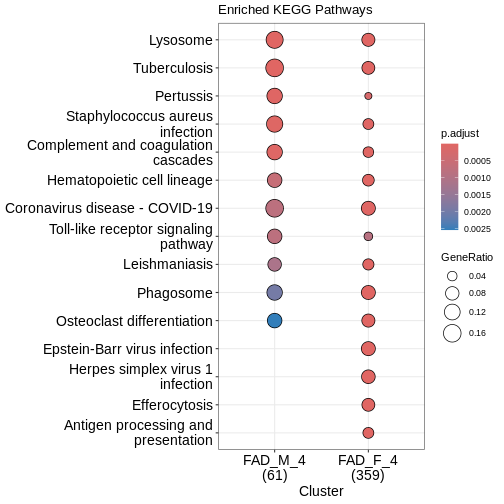
What does this plot infer?
Save Data for Next Lesson
We will use the results data in the next lesson. Save it now and we
will load it at the beginning of the next lesson. We will use R’s
save command to save the objects in compressed, binary
format. The save command is useful when you want to save
multiple objects in one file.
R
save(DE_5xFAD.df, DE_5xFAD.list, file = "results/DEAnalysis_5XFAD.Rdata")